FBP Nbox walkthrough
1. Process the raw NMR data
Eleven titration points were acquired in this series of experiments. The protein and ligand concentrations ('P0' and 'L0'), together with the number of scans ('ns') an receiver gain ('rg') used in the NMR acquisition, are tabulated below. FBP Nbox titration parameters:
11 1H,15N-HMQC experiments have been recorded as part of this titration experiment (directories 1-11). A script, 'proc-all.com', is provided to process these in a uniform manner with NMRPipe. Note that several of the parameters in the above script will be required when setting up the 'virtual spectrometer' used in the TITAN analysis:
- 600 MHz field strength (base frequencies 599.927 MHz and 60.797 MHz)
- 15N carrier frequency is at 118.959 ppm, with a sweep width of 1823.985 Hz or 30 ppm
- data are processed with exponential window functions (4 Hz in the direct dimension and 8 Hz in the indirect dimension)
- 128 complex points ('td = 256') in the indirect dimension, doubled to 256 with linear prediction and doubled again to 512 by zero filling
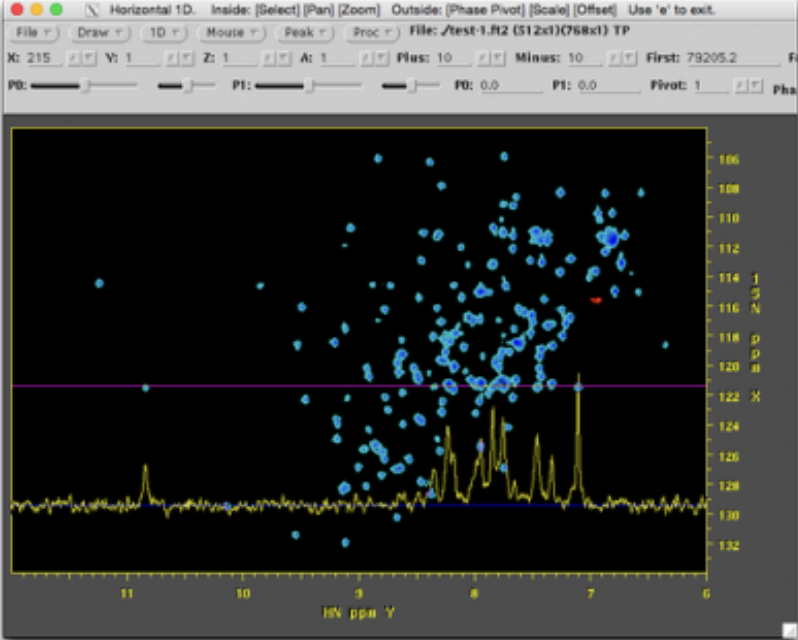
Run the script now to process the data, which should make 11 files 'test-1.ft2' to 'test-11.ft2'. Examine the spectra in nmrDraw to make sure they're been processed and phased correctly.
- an ROI must be selected in each spectrum
- estimates of chemical shifts must be provided for each state in the binding model
- estimates of linewidths must be provided for each state in the binding model (although generally the default values of 20 s-1 provide an acceptable starting point)
- overlapping peaks that should be fitted simultaneously should be marked as belonging to the same 'spin group'. Spin groups can be given any label you like, or just left empty to fit the spin by itself.
- Using only the first spectrum (recorded in the absence of ligand), fit only chemical shifts and linewidths for the first state of the binding model (i.e. free protein).
- Now use all the spectra to optimise the chemical shifts and linewidths of the second state (i.e. bound protein), together with the model parameters (Kd and koff).
2. Launch NMR TITAN
Option 1. Install and run the TITAN app directly.
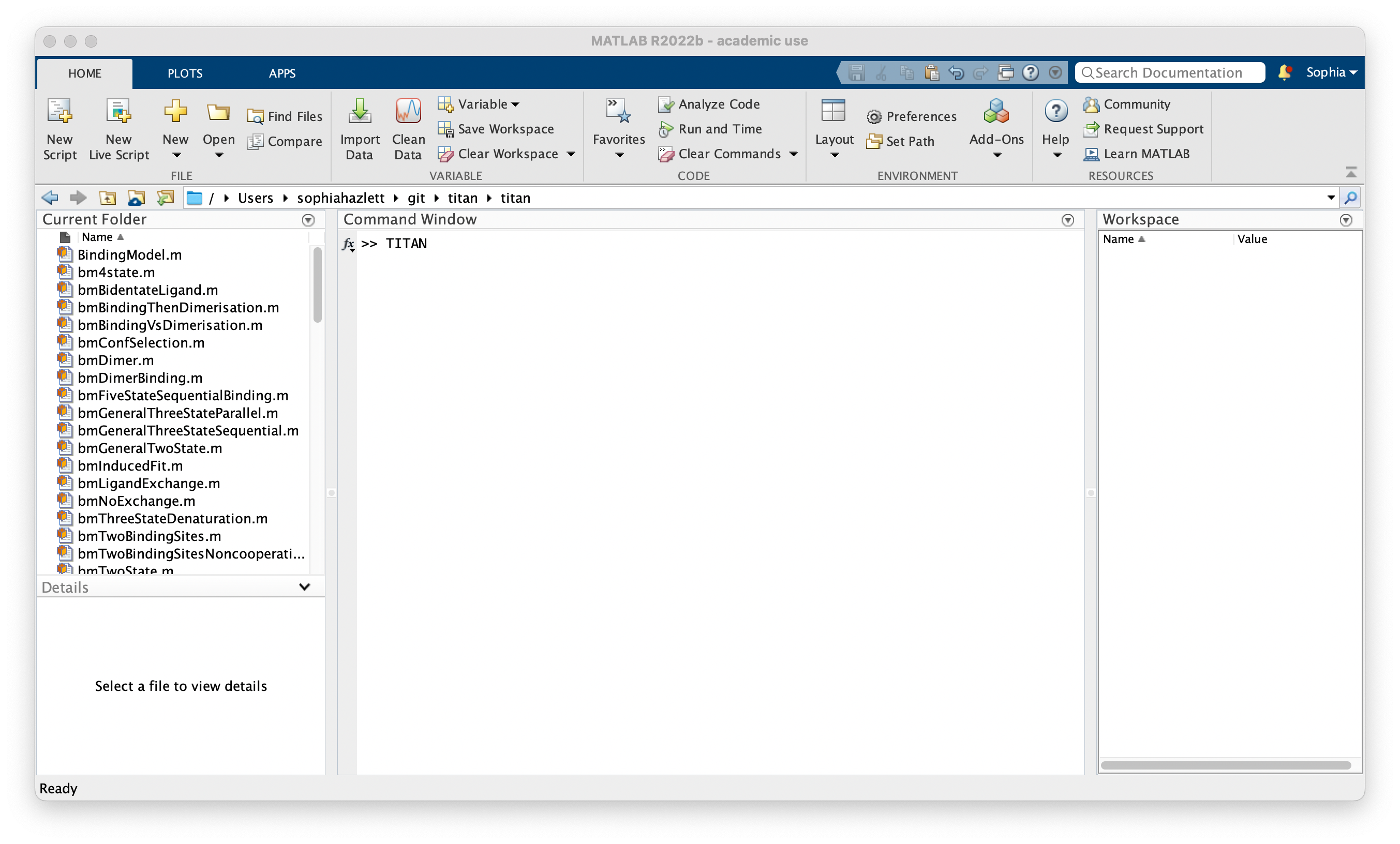
Option 2. Run the TITAN app from within MATLAB.
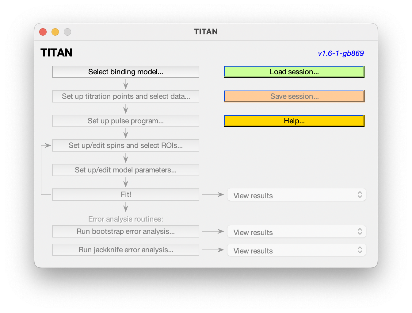
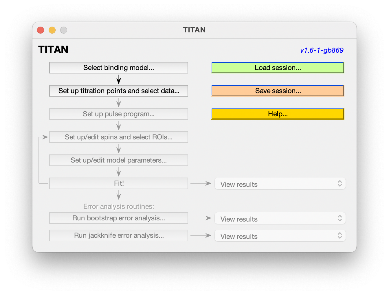
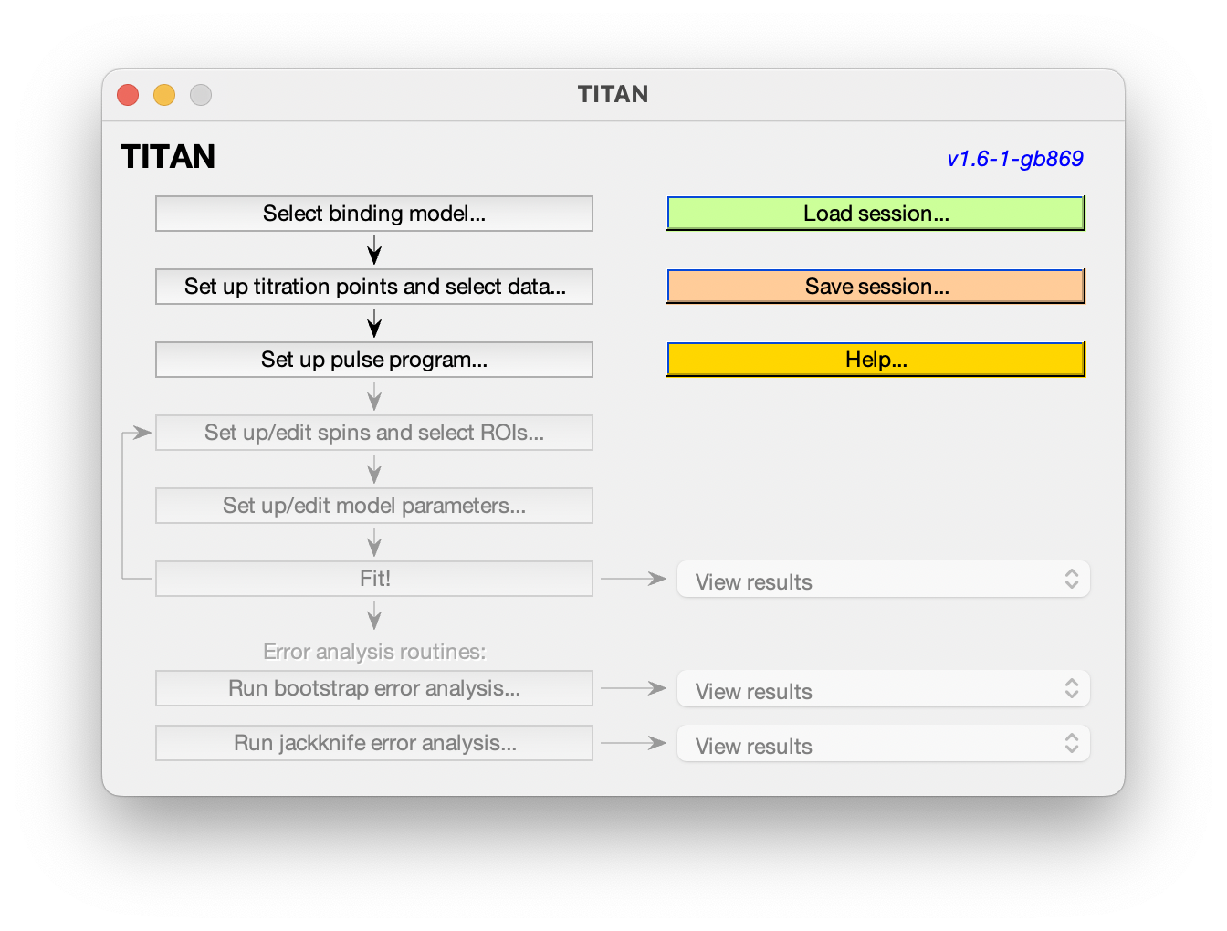
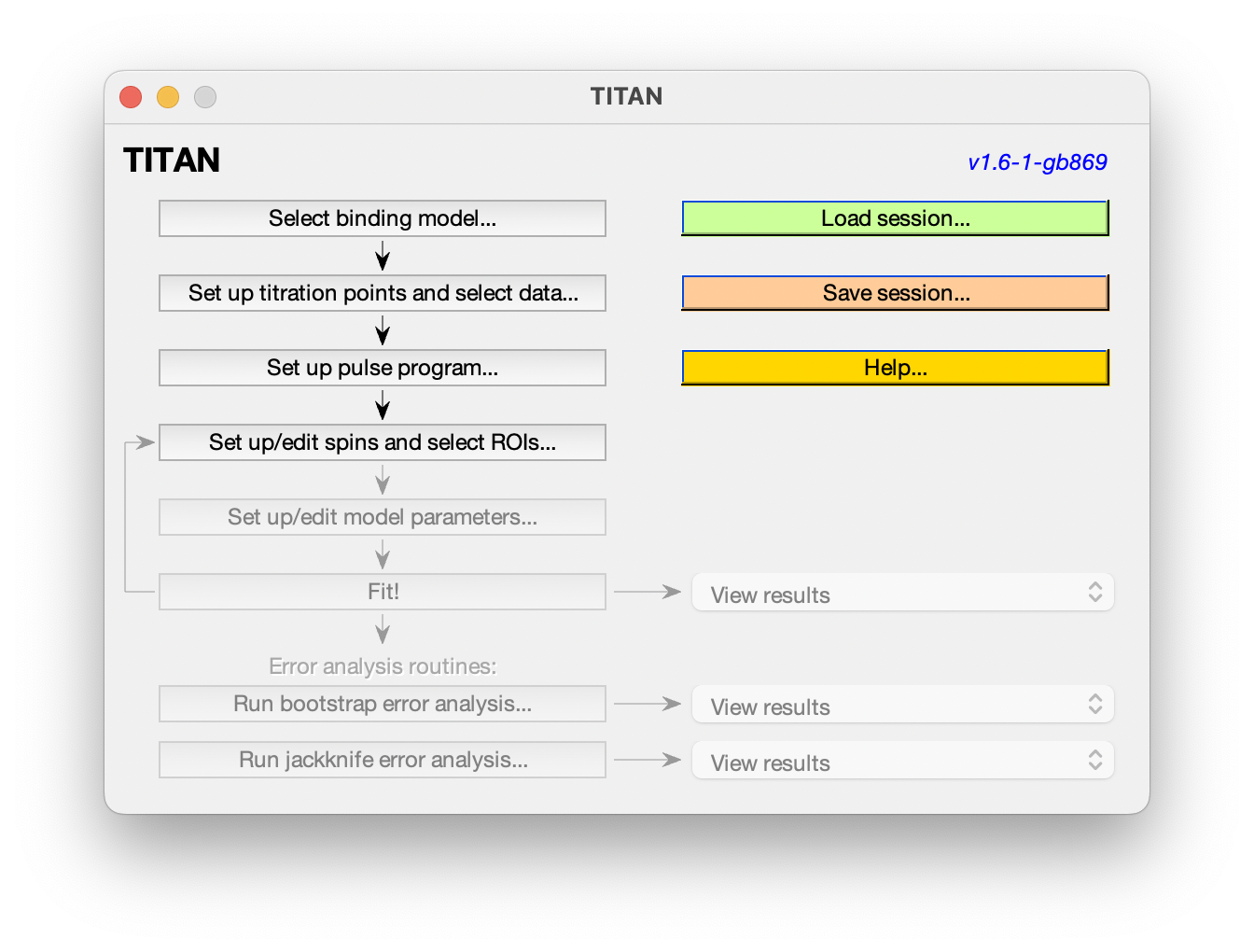
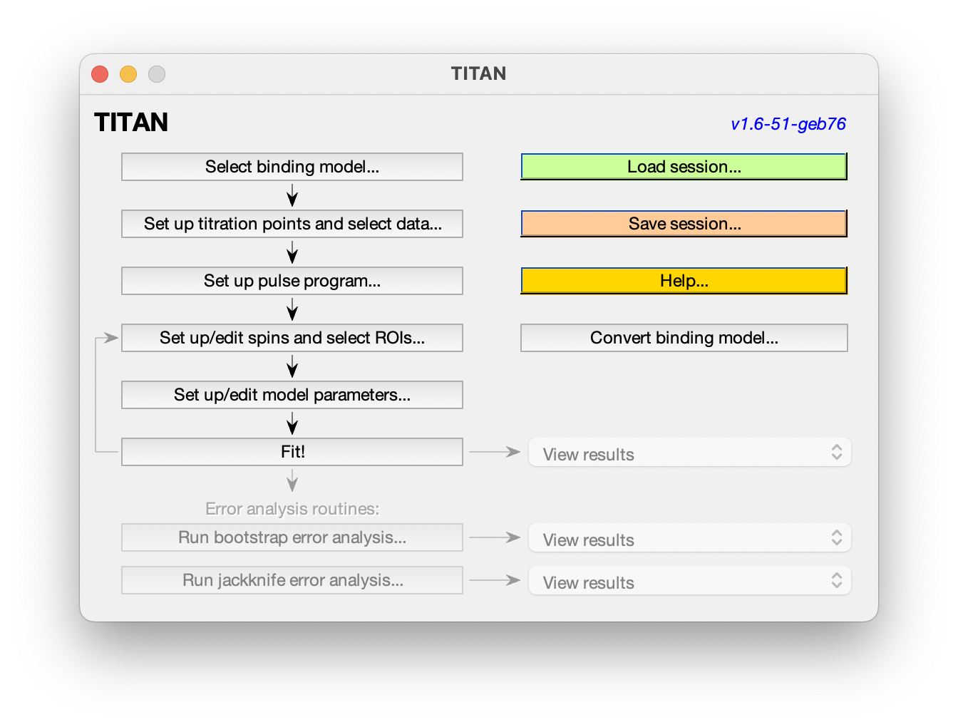
Start the main TITAN graphical user interface with the command 'TITAN'.
The main interface shows the analysis pipeline. Commands will become enabled as you progress along the pipeline. At any point, you can load or save the current session, and some example sessions are also provided to explore.
3. Select a binding model
TITAN is designed with a flexible core of simulation and fitting routines, which can be combined with a variety of pulse programs and binding models.
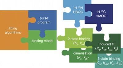
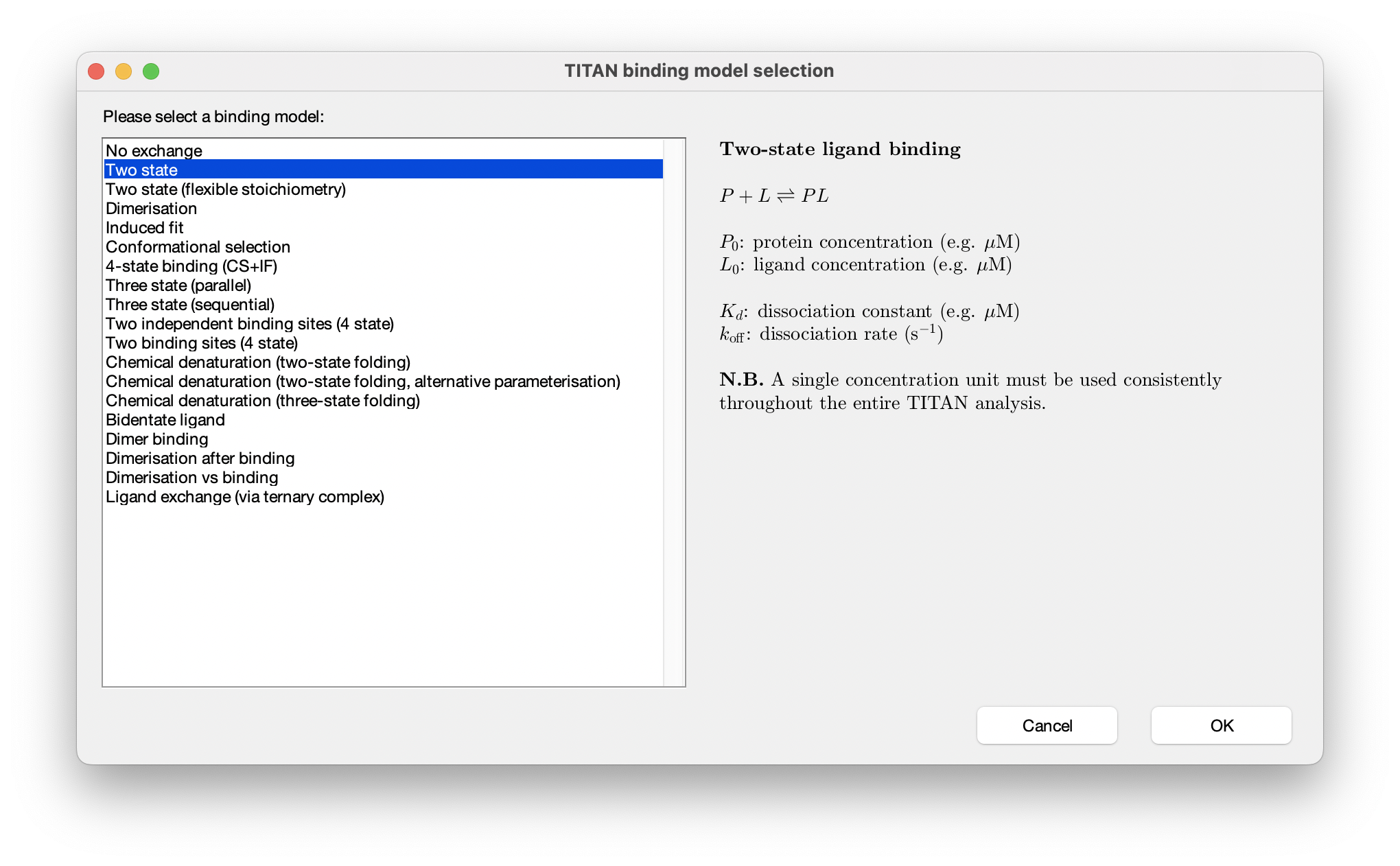
Binding models are objects such as Kd values that represent chemical behaviour of species , and which tranlsate concentrations and model parameters such as Kd values into exchange rates of NMR calculations. A variety of binding models are available. Here we're going to use a two-state model, which describes the simple binding process: P + L ⇌ PL.
Choose Select a binding model... and select the two state model from the list of built-in models:
4. Set up titration parameters, and load experimental data
Once a binding model has been selected, the next step in the pipeline will be enabled:
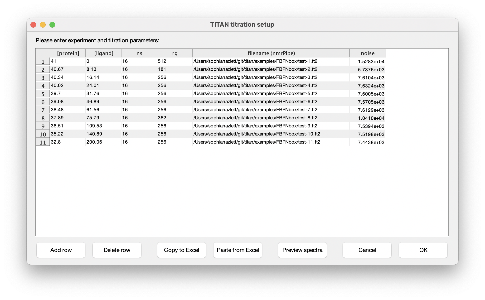
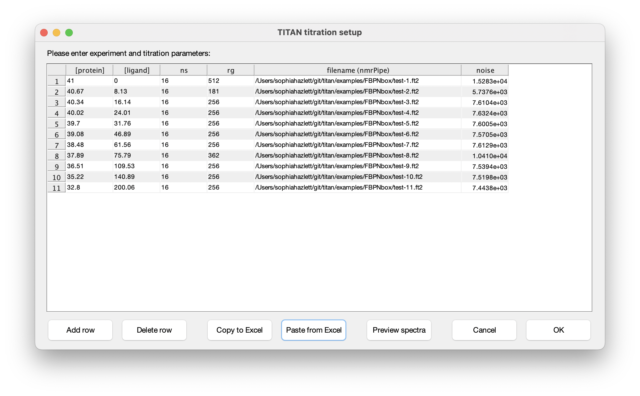
Choose Set up titration points and select data... to bring up the titration dialog:
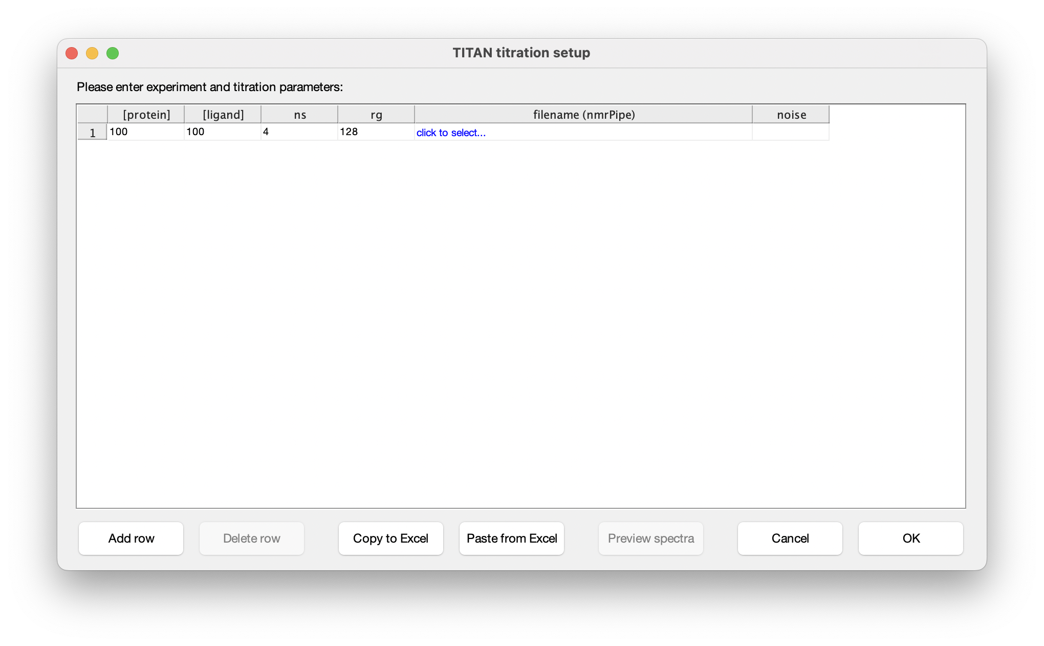
The columns in this table depend on the binding model. In this instance, protein and ligand concentrations need to be specified, together with NMR acquisition parameters and the location of NMRPipe format data files (as processed earlier). Either fill in the table cell by cell, or paste the entire contents at once from the clipboard. Note that the paste function will overwrite the entire table of contents. On selecting a data filename, either manually or by pasting from the clipboard, TITAN will automatically calculate an estimate of noise in the spectrum (based on maximum likelihood estimation of a truncated Gaussian distribution, using ca. 80% of the observed data, excluding intense regions associated with peaks). This can be manually overwritten if necessary. Note that accurate noise levels are critical for correct weighting of residuals across multiple spectra.
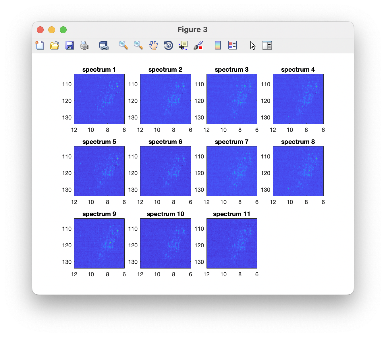
Plot the data to verify a successful import
The imported spectra can be quickly plotted as intensity colourmaps using the Preview spectra command:
5. Prepare the pulse program for the 'virtual spectrometer'
Once titration points have been prepared, the next step is to select and set up a pulse program for the simulation.
Pulse program objects contain the code to simulate the evolution of magnetisation for a given experiment type. They must be initialised with experimental parameters such as magnetic field strength, spectral width, number of points, etc. Once prepared with these acquisition parameters, the pulse program can be plugged into the simulation and fitting routines, together with a binding model prepared above.
In this set of measurements, data were acquired using a 1H,15N-HMQC experiment:
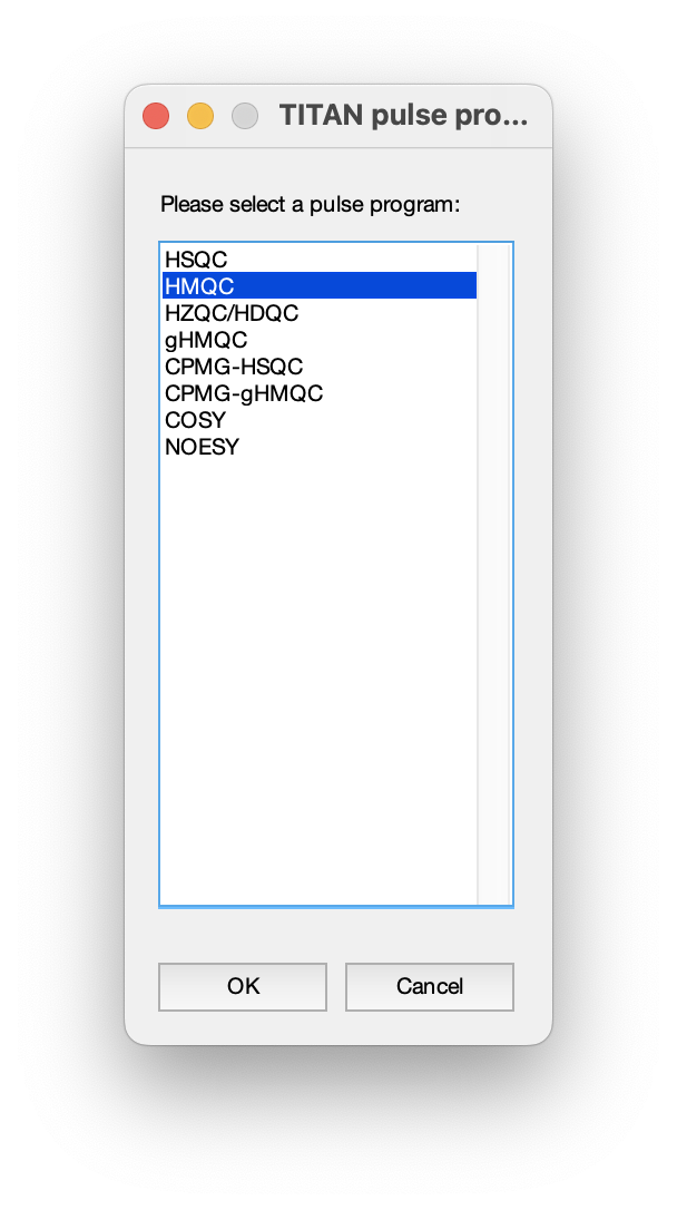
Once selected, a number of acquisition parameters must be specified. Most of these should be correctly determined from the imported NMRPipe data, but note particularly that the scalar coupling constants must be specified by hand:
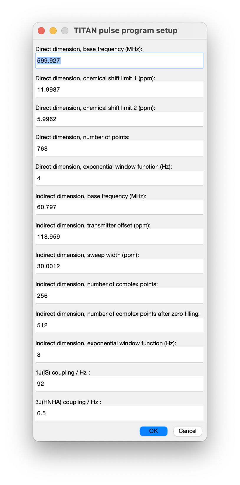
6. Set up spins, regions of interest (ROIs) and initial peak positions
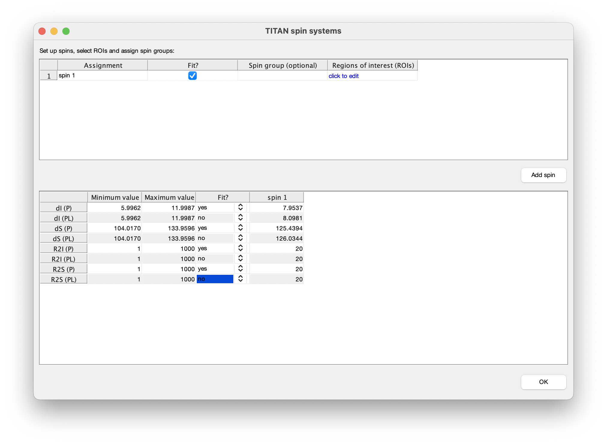
For every spin system (residue) and every spectrum a region of interest (ROI) must be defined to select the datapoints used for fitting. Each spin system is represented in TITAN by sets of direct (I) and indirect (S) spin chemical shifts and linewidths (R21, R2S). Each state specified by a binding model must have chemical shifts and linewidths associated with it, and initial estimates of these must be provided before fitting.
So, when adding a residue to be fitted, several things need to be set up:
A simple interface is provided for curating lists of spins, and selecting/editing ROIs and initial spin system positions. Upon opening this for the first time, you will immediately be prompted to select a ROI to create a new spin system:
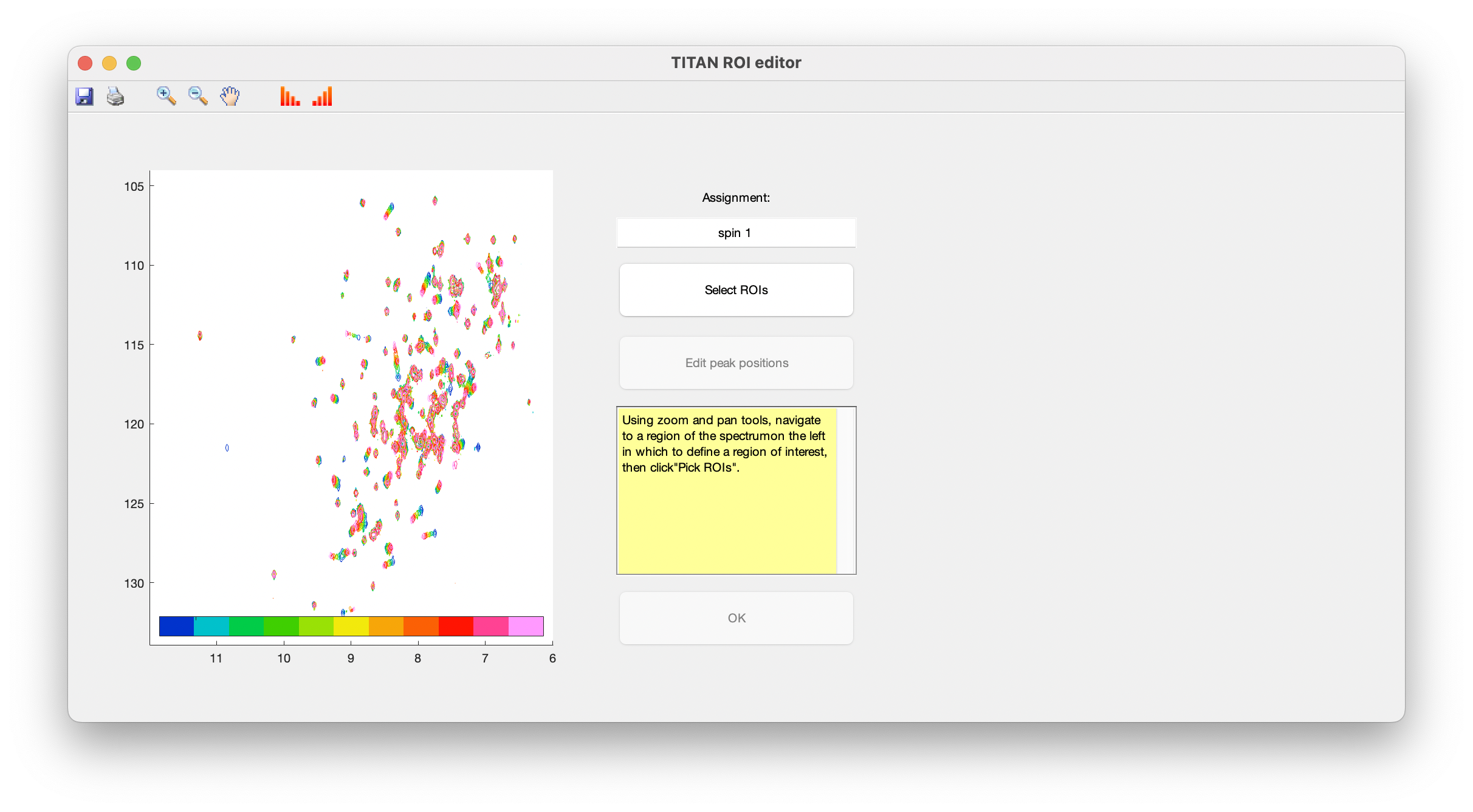
Use the zoom and pan tools from the toolbar to center the view on a residue showing interesting exchange behaviour, then choose Select ROIs to begin the process of marking out ROIs.
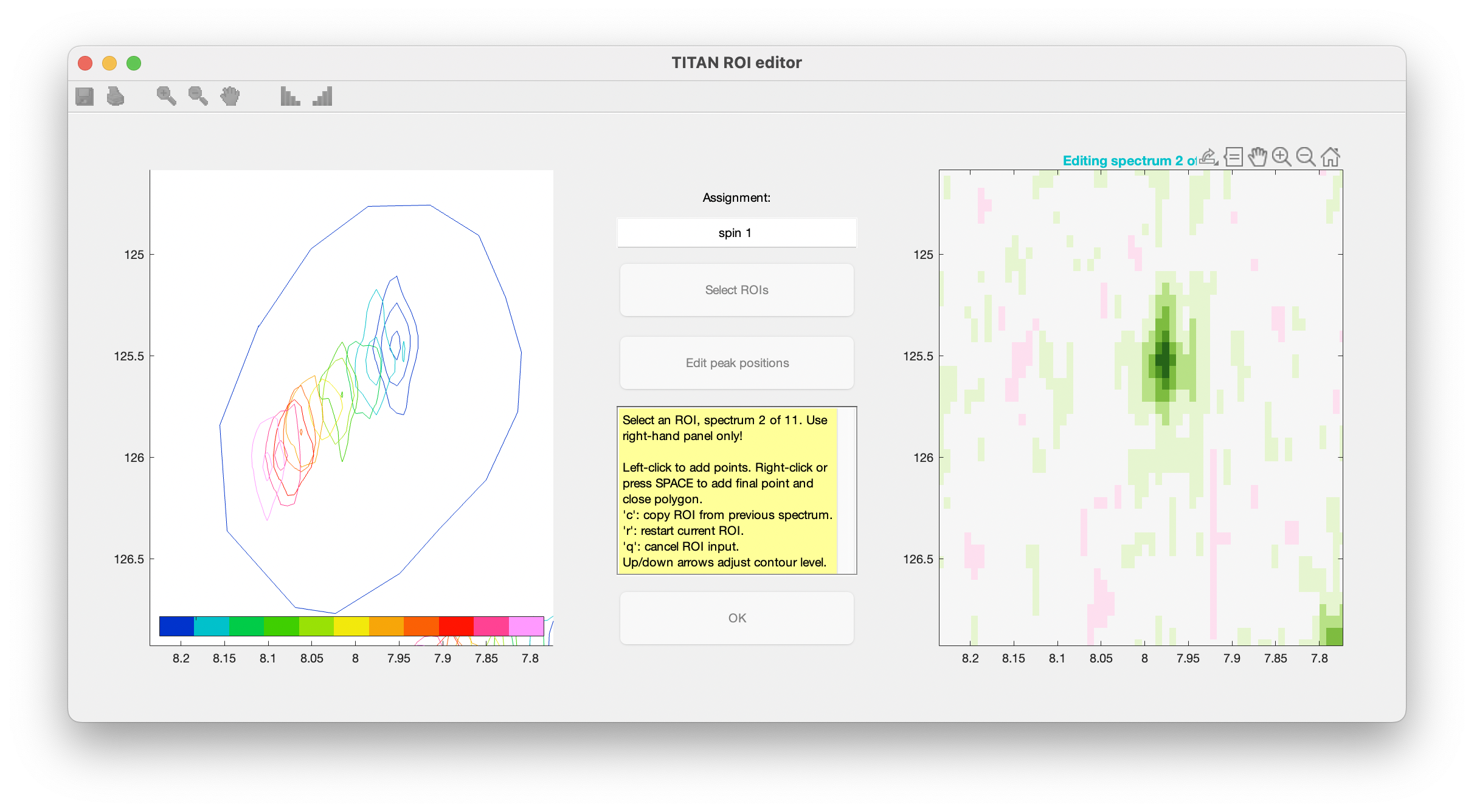
ROIs are specified as a series of polygons enclosing the data to be fitted. The TITAN interface will display density plots of each spectrum in turn in a right-hand panel, in which the mouse should be used to mark out the ROI.
When complete, use the right mouse button or press 'SPACE' to add a final point, close the polygon, and move on to the next spectrum in the series.
Continue this process for each spectrum in the titration series. The shortcut 'c' can be used to copy the ROI marked out in the previous spectrum.
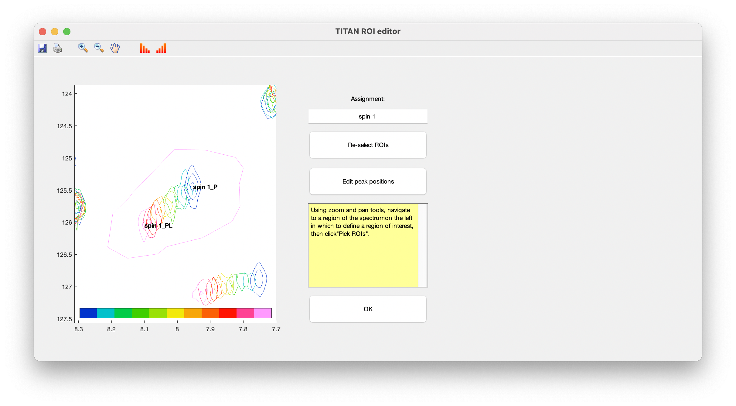
When an ROI has been selected for the final spectrum, you will be prompted to provide initial estimates of peak positions for each state in the binding model (i.e. free and bound protein), by left-clicking in the left-hand panel:
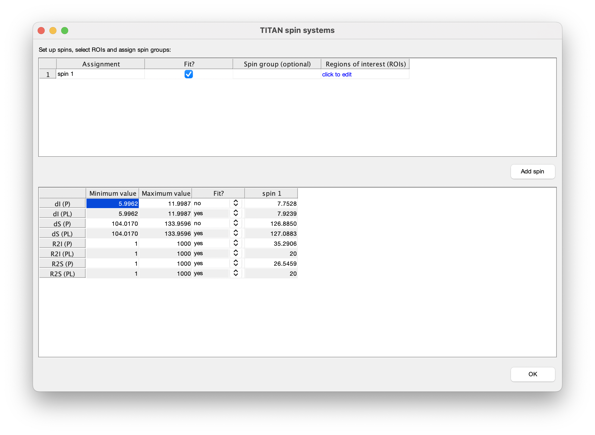
Once complete, close the dialog to return to the list of currently defined spins. The links in the top panel can be used to return to the ROI editor, and to include/exclude the spin from any fitting process.
Preparing for fitting
Because there are so many free parameters around, it's important to constrain them as much as is reasonable, to try and prevent the volume of parameter space exploding. Here, we take a 2-step approach to the fitting problem:
The bottom panel in the spin editor provides control over which parameters should be optimised in the fitting process. In accordance with the strategy above, select to only fit parameters associated with the free state of the protein:
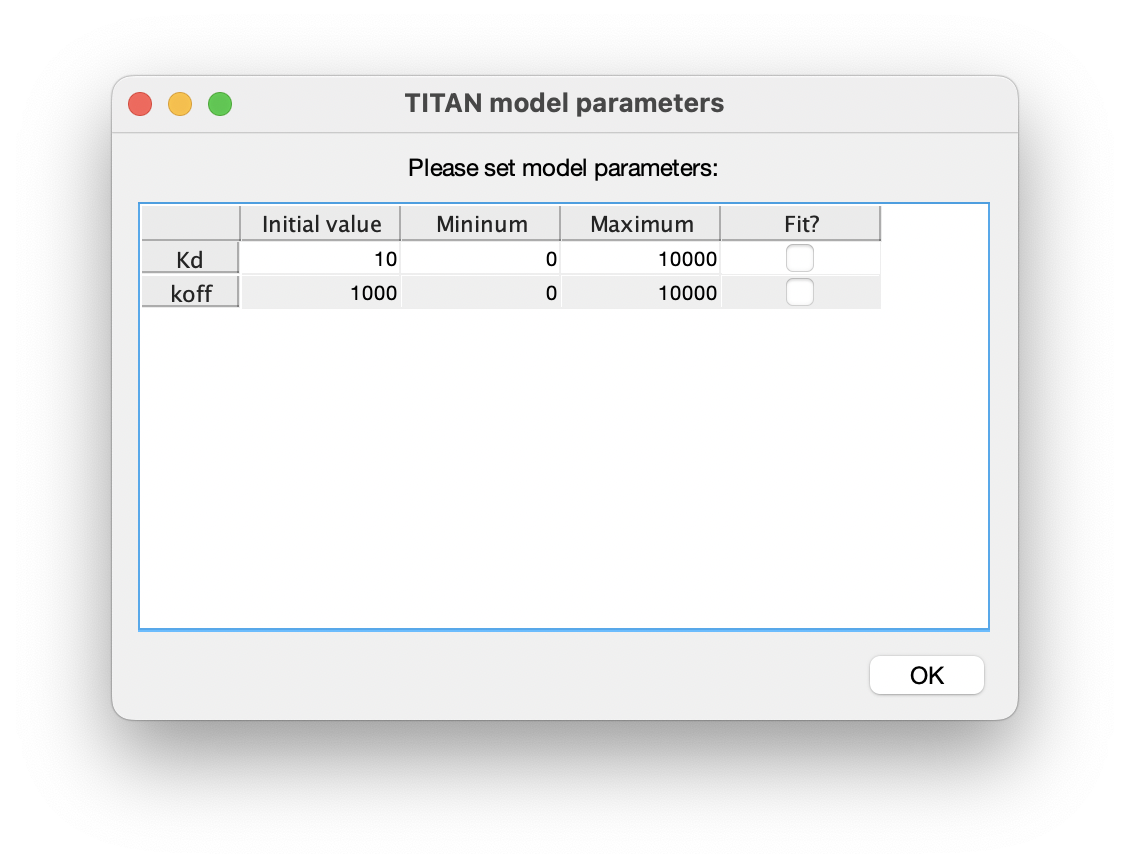
7. Set up model parameters

8. Fitting 1: Fit only the free state using the first spectrum
The Fit! command should now be enabled:
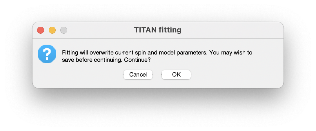
The fitting process will use the current set up as a starting point, but these values will be overwritten by the new fitted values. It's a good idea to hit "Save session..." at this point so you can go back if necessary.
When choosing Fit!, you'll be presented with a warning as a reminder of this:
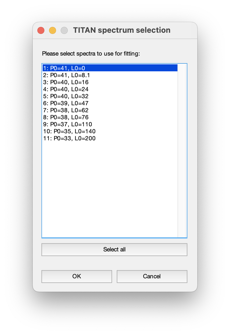
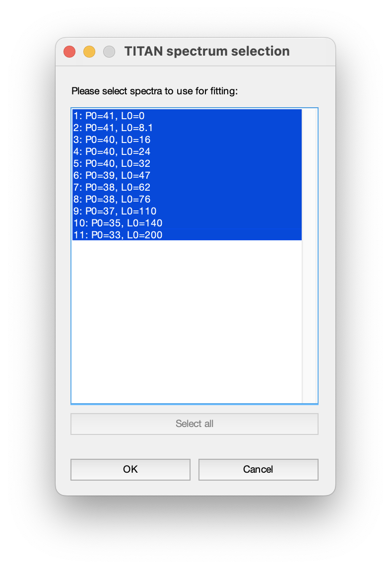
After accepting this warning, you will be prompted to select the spectra to be used in the current fit. For this first step, we only want to use the first spectrum:
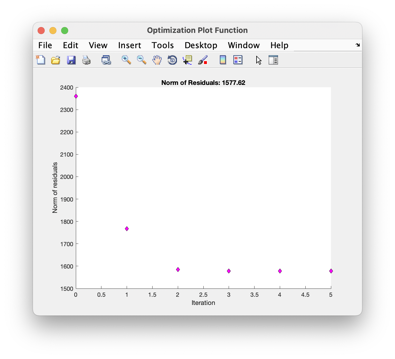
Fitting outputs
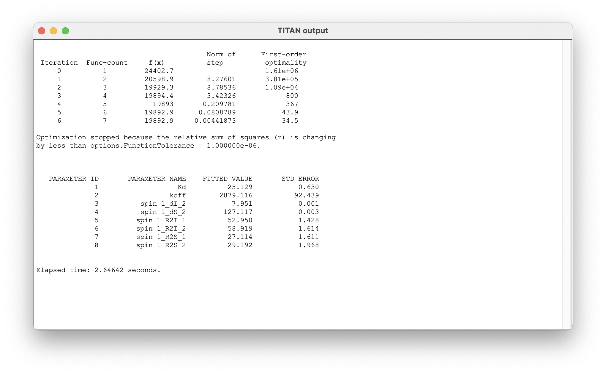
While running, a plot of the chi-square residuals is displayed to show the progress of the optimisation algorithm:
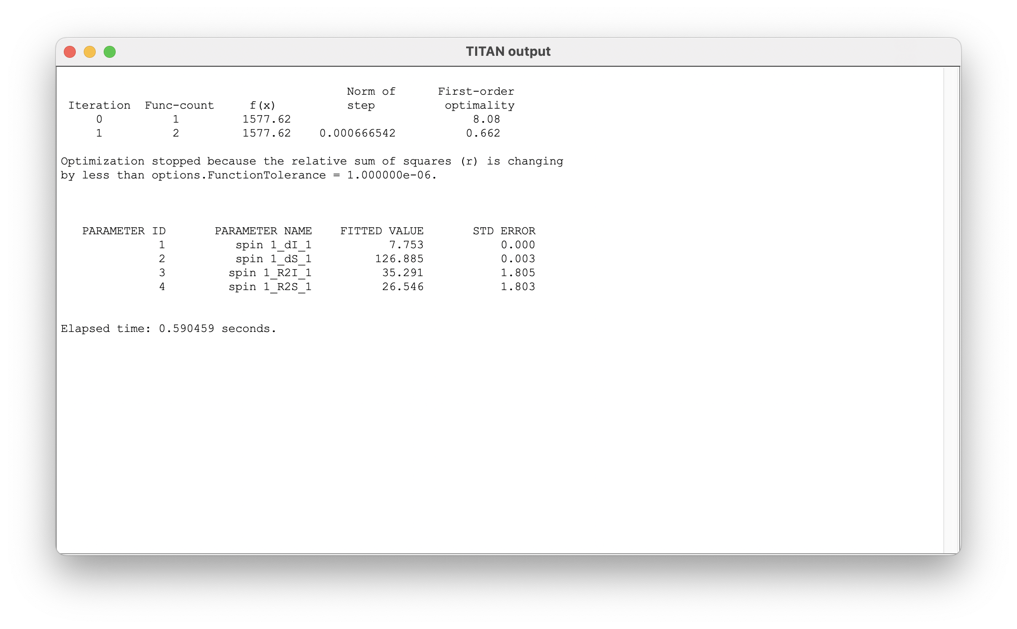
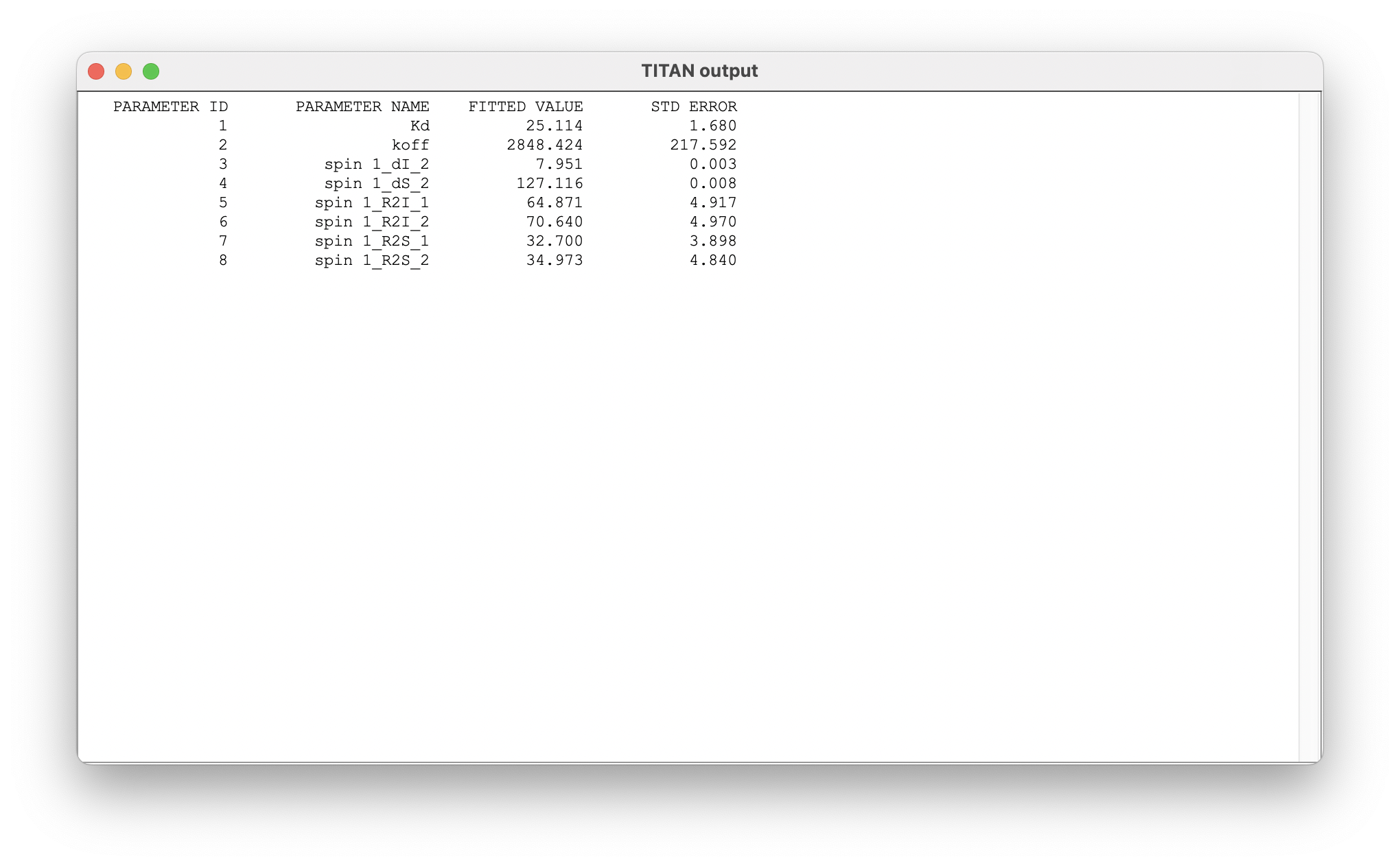
On completion, a list of the fitted parameters is displayed in a new window. Parameter labels are of the form: 'ASSIGNMENT_QUANTITY_MODEL STATE'. Note that the reported error comes from the estimated covariance matrix - the use of bootstrap resampling methods (below) is recommended for more robust estimates.
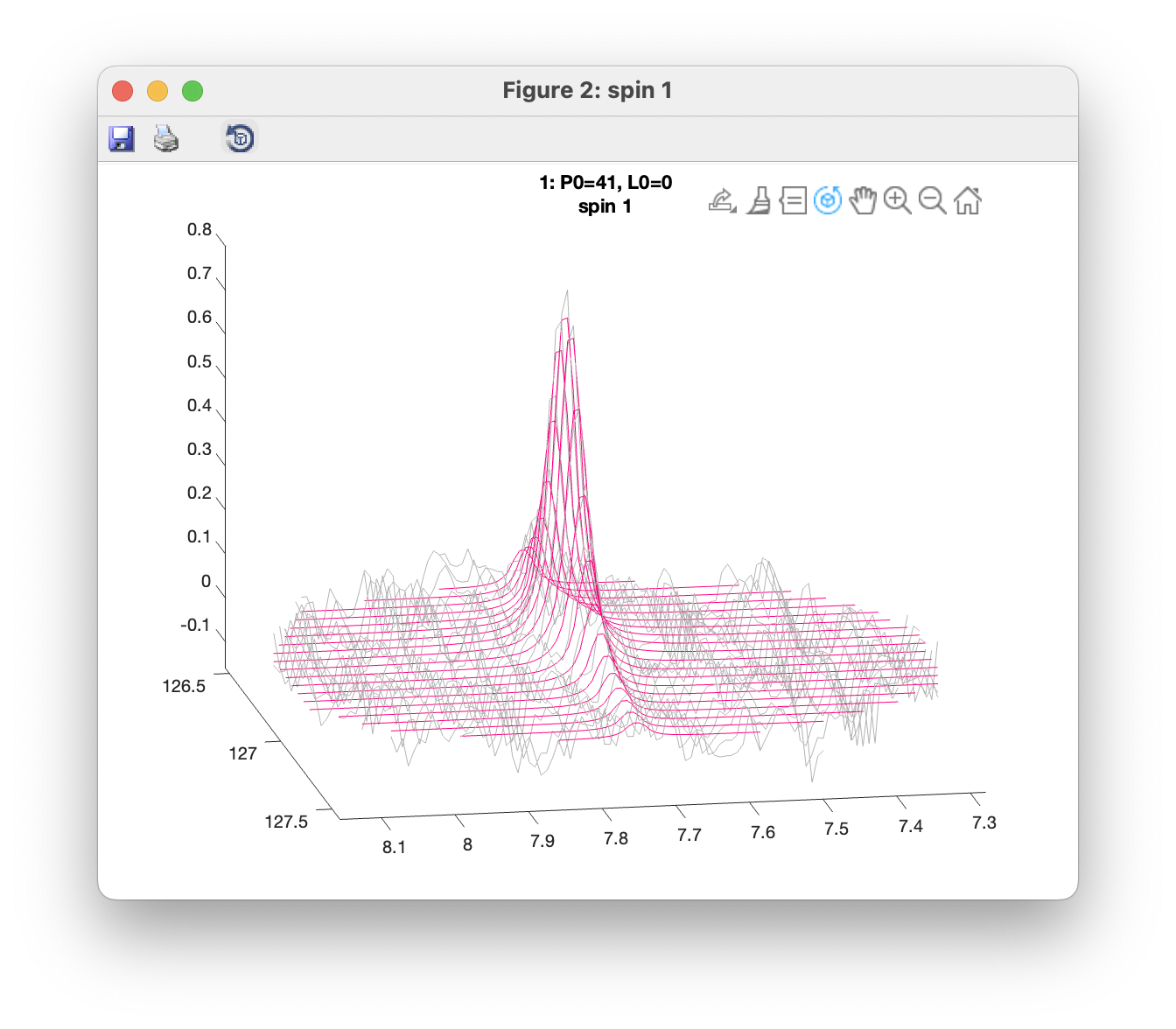
A number of options are provided to plot the fit results:
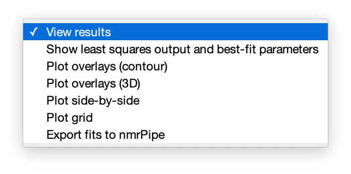
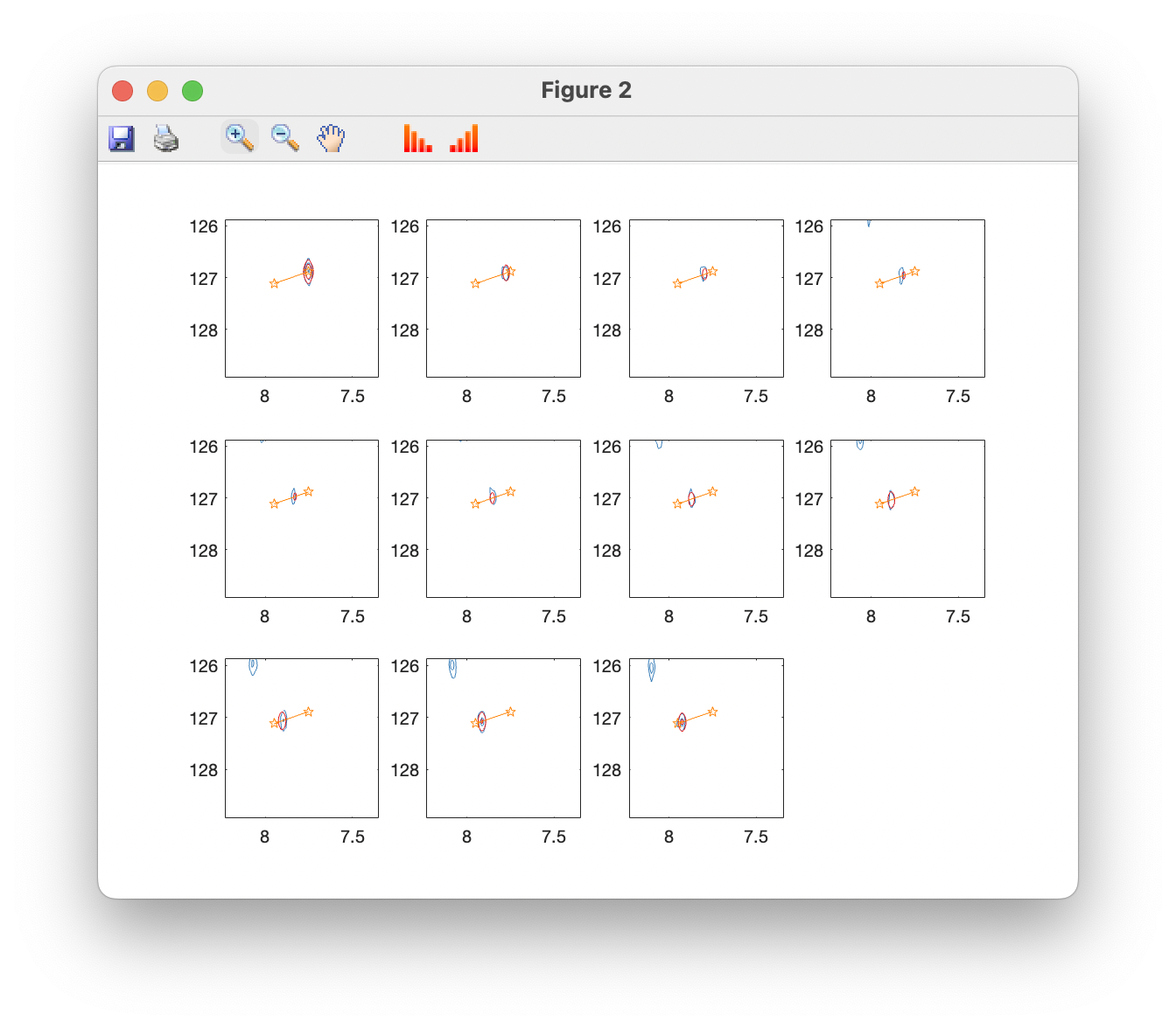
Plot overlays (contour) opens a window showing the original spectrum in blue, with fits superimposed in red, and fitted peak positions in orange. You can use the standard zoom and pan tools to examine peaks more closely, and toolbar buttons can be used to raise and lower the contour levels:
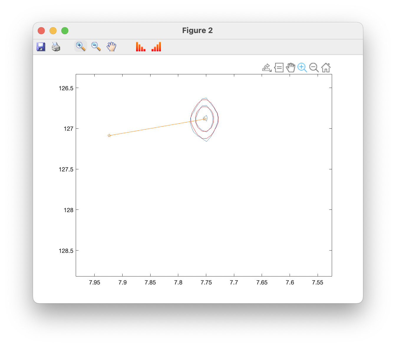
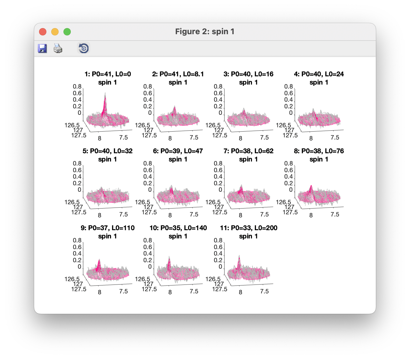
Plot overlays (3D) opens a window showing a 3D view with observed data plotted in grey, and fitted data in red. Separate windows are opened up for each spin group. Only data within the defined ROIs are shown. 3D views can be rotated using the Rotate 3D tool.
9. Fitting 2: Fit the bound state and model parameters using all spectra
We use the results of the previous fit as a starting point for second fitting step. Return to the spin editor, and turn on fitting of bound chemical shifts and all linewidths.
Similarly, turn on fitting of the model parameters 'Kd' and 'koff':
Now run the fitting process again, using all the spectra:
The fit results now provide estimates of the model parameters, as well as bound state chemical shifts:
Fitting outputs
Contour plots are now shown for all spectra in the titration series:
As do 3D plots:
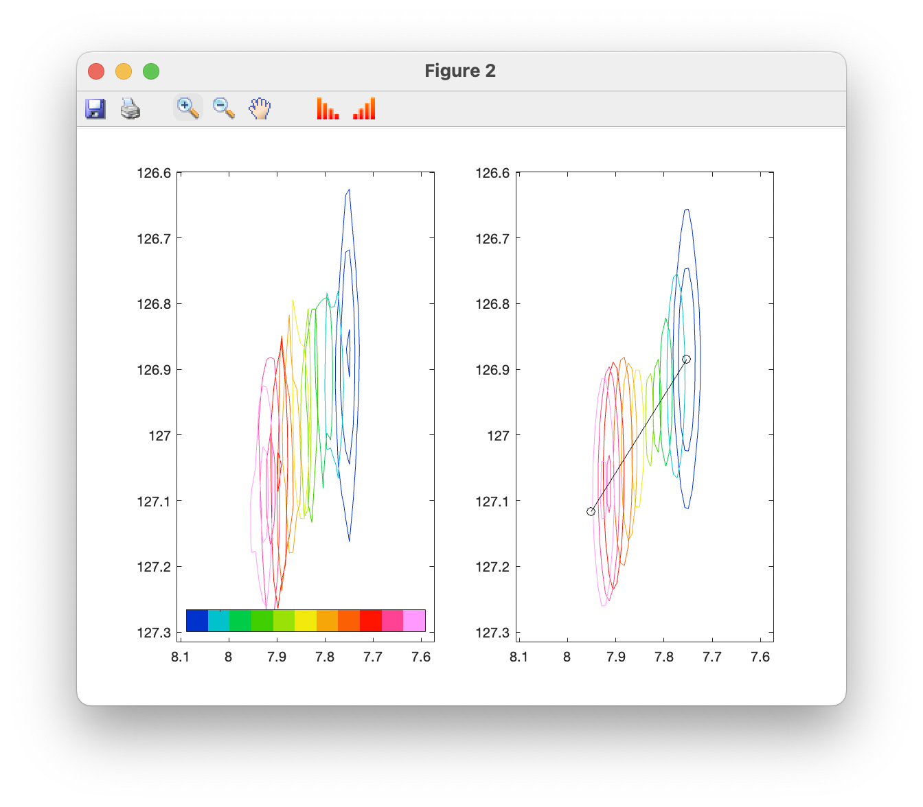
A side-by-side plot of observed and simulator spectra can also be produced:
10. Error analysis by bootstrap resampling of residuals
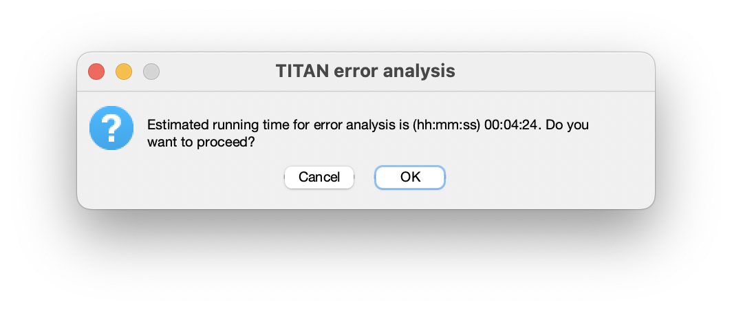
Once the fitting has been completed, the option to run a bootstrap error analysis will be enabled. This will repeat the previous fitting step, using the same starting parameters as before, based on resampling of residuals from the best- fit spectrum. To run, enter the number of resampled spectra to be generated.
An estimate of the running time will be displayed, based on the time required for execuation of the original fit:
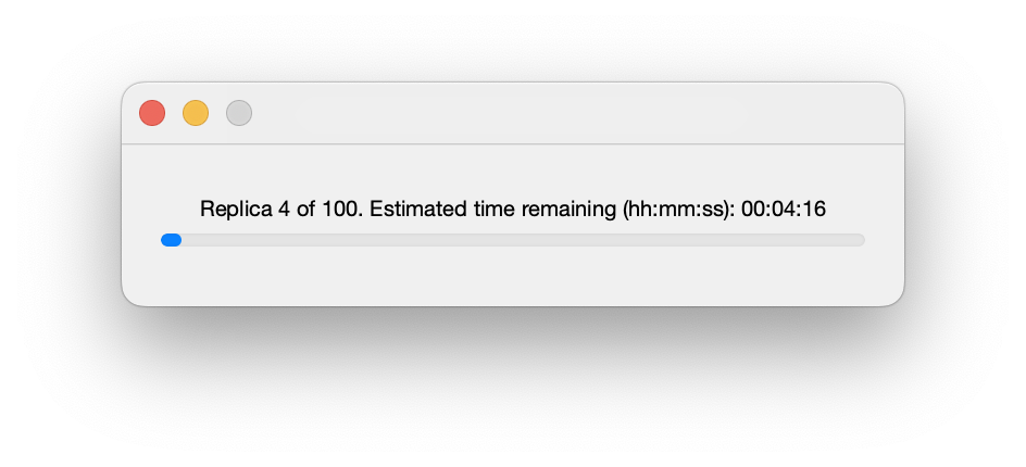
Once running, a progress bar shows the current status of the calculation. Closing this window will halt the calculation after completion of the current fit (but note that for complex fits this may take many minutes!):
Once complete, a number of results may be displayed:
The summary of results shows the mean and standard error of parameters determined from the bootstrap analysis.
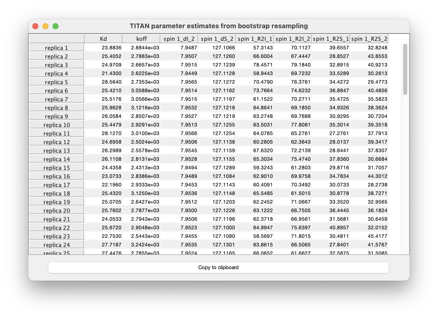
Results of each individual fit may also be tabulated:
Finally, the correlations between estimates of various parameters may be investigated via the covariance matrix. The data cursor may be used to explore points of interest. In this case, we observe that estimtes of the Kd are strongly correlated with the bound state chemical shift:
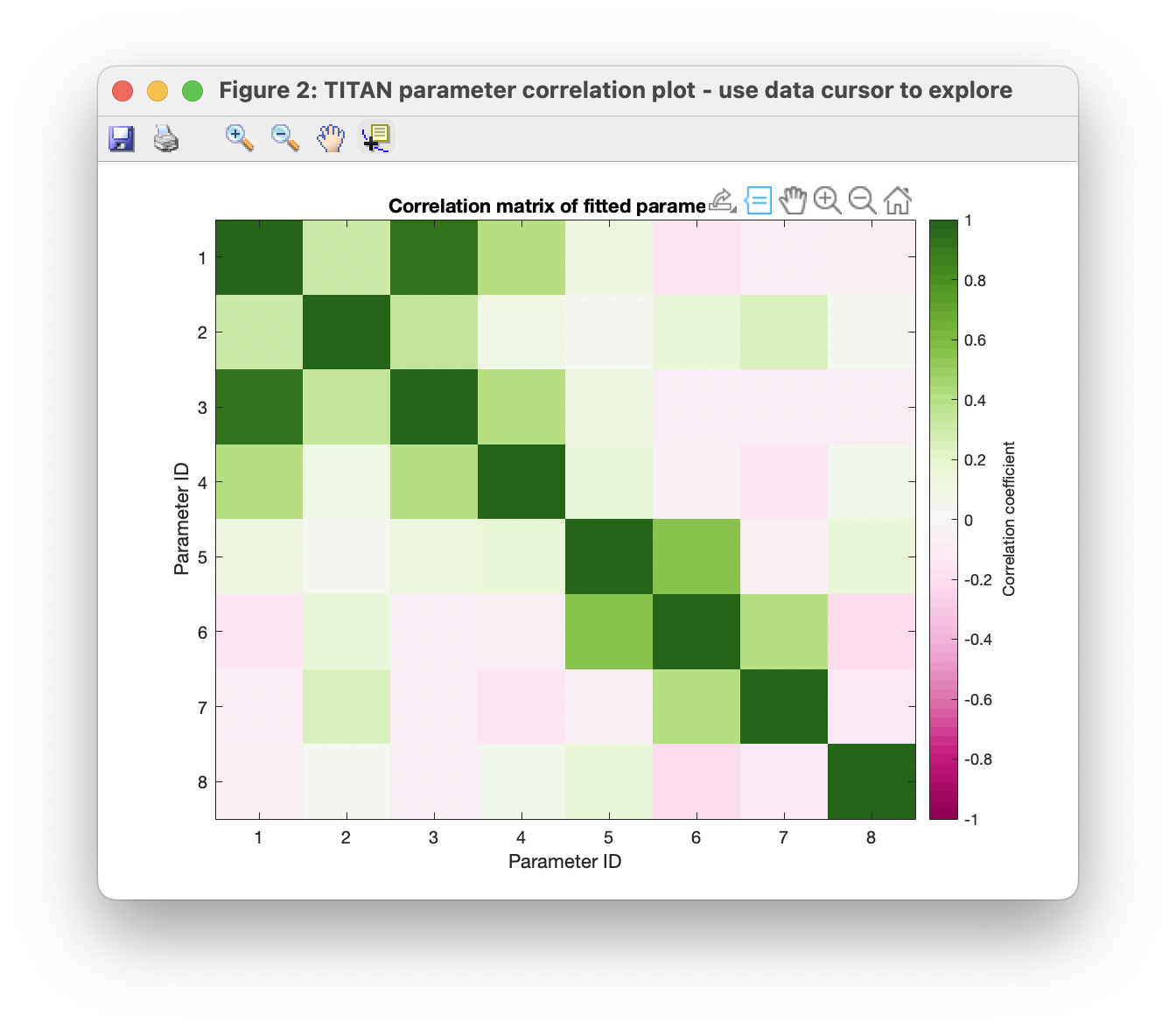
Upon a more detailed analysis with many more spins however (e.g. the provided example 'TITAN_session_fitted.mat', based on global analysis of 25 spins), the covariance structure may be improved.